3D Grande Prairie Buildings (LiDAR)

Sometime in the last year, the County of Grande Prairie (Alberta) starting providing bare earth and full feature LiDAR through their Open Data Catalogue (LiDAR download map here). Here’s how you can use the data to visualize 3D buildings, using a combination of ArcGIS for Desktop (with Spatial Analyst and LAStools), QGIS, and Cesium JS.

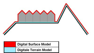
1. Find and download the bare earth (digital terrain model = DTM) and full feature (digital surface model = DSM) LiDAR zip files for a quarter section of your choice from the LiDAR viewer (I used the files here and here). To familiarize yourself with the concepts of DSMs and DTMs, read this answer.
2. Download LAStools and add the LAStools toolbox to ArcMap (or ArcCatalog)
3. Run the las2dem tool within the LAStools toolbox for each of your downloaded .las files. You can accept all default parameters.
4. The tool should output a .tif image for each surface, projected to UTM Zone 11. If not, run Define Projection to assign the projection.
5. The names of each layer will be the same, by default (e.g. “710622NW.tif”). Change them to be unique, so geoprocessing tools (and you) can easily tell them apart (e.g. “710622NW_BE.tif” and “710622NW_FF.tif”).
6. The DTM and DSM each report elevations in meters above sealevel. Since we are interested in the difference between those elevations (i.e. the difference between rooftop and the ground pixels) we need to subtract the two images. You can do this using the Minus tool, or more generally, Raster Calculator. I used the expression: Int(“710622NW_FF.tif”-“710622NW_BE.tif”) to return the difference between the DSM and DTM, as integer numbers (this will simplify things later on).
7. Eventually, we are going to want polygons to load into Cesium (on the order of hundreds or perhaps a few thousand), not individual pixels (there are 700,448 pixels in my image). At this point, we have what is called a classified image, classified by height in meter increments. We want to group this classified image by similar height values, and we can do that by processing our classified output. Following the instructions in this link, we are guided through filtering, smoothing, and generalizing our output.
8. Run Raster to Polygon on your generalized output to produce polygons.
9. Cesium is going to want lat/long coordinates, so you may as well run the Project tool on your polygons to switch the data to WGS84.
10. As far as I know, ArcGIS does not support GeoJSON (which we are going to use in Cesium). Conveniently, QGIS does. So, load your polygons in QGIS and “Save As…” GeoJSON.
11. Upload your GeoJSON to your host.
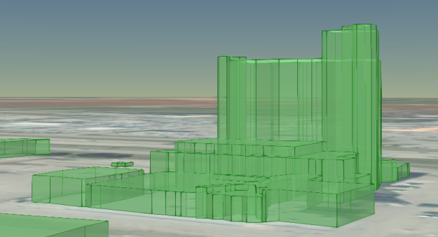
12. Switching to Cesium, create a map and load your GeoJSON (general example here). Cycling through the GeoJSON polygons, assign the polygon height to 0, and the extruded height to match the elevation attribute in your data (for me, that was stored in the “GRIDCODE” field).
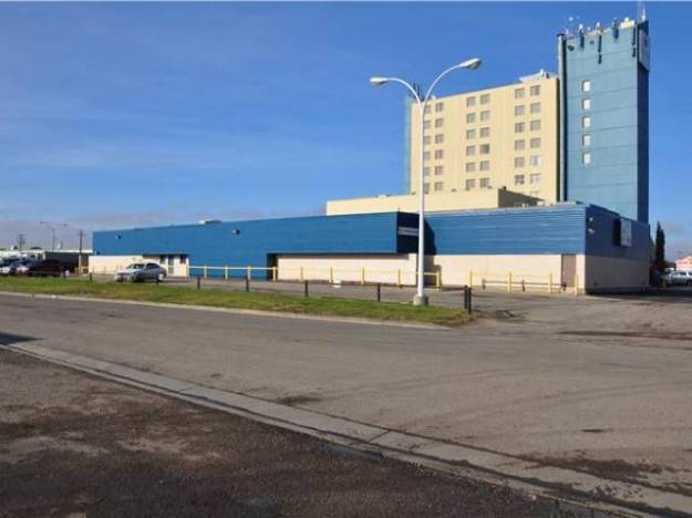
13. That’s it! You can see my interactive example here, using a “modern” browser. Here’s a sample, showing the Paradise Inn (pictures from my example, and Tom Shield Realty):

Note: I tried and failed to add a link to the LiDAR Open Data License in my example. Hopefully, this will be sufficient.

 

 

Little Bobtail Lake Fire: Before/After

You may recall the Little Bobtail Lake fire in the Prince George, BC area that burned over 25,000 ha in 2015 (curious to compare 25,000 ha to your area? Check here).

How does it look now? Did the fire burn and kill the entire area? These are some questions that can be explored quite easily now using archived and processed imagery from Astro Digital. I’ve made an example for the Little Bobtail Lake fire here that compares imagery from before the fire (April 9, 2015) and after the fire (June 28, 2015), and here are the steps I used to do it:

1. Sign up for a free Astro Digital account here.
2. Sign in and you’ll find yourself at “Mission Control”.
   1. Start a new “task”.
   2. Edit the task.
   3. Select the images you want to process
   4. Submit the task, choosing web map as the output. I wanted true color (visual), false color (mostly land vs. water differentiation), and NDVI (for vegetation health. Green = healthy vegetation, blue/black = dead/dormant/non-vegetated) images, so I chose all of those options.
   5. Submit the task and wait for the images to be processed.
3. Once the images are ready, follow the instructions for Using Processed Imagery via Mapbox. You need to use Astro Digital’s public Mapbox key to access the web map imagery. I believe it would be possible to download the raw imagery from Astro Digital and make tiles yourself to upload to your own Mapbox account, but I have not done that here. The tradeoff is that Astro Digital limits the key to 100 map views/web page, so if this map is unavailable, you can rest assured that it has gone viral (yay me), so try back tomorrow.
4. That’s it! The map is here. Try it out. Toggle the layers on and off – “on” layers at the top of the list cover up those underneath, so you need to turn off the upper layers to see the lower layers. Try flipping back and forth to see the difference in NDVI layers – notice that before the fire, the Little Bobtail Lake area looked just like the surrounding area (it’s dark because the vegetation is still coming online after winter), while after the fire, the results are quite striking. Have fun!

Inspiration: AstroDigital blog, Mapbox examples

 

Nechako Aquifer & Wells

Curious where the Nechako Aquifer is located, now that a new report (article) has indicated that a hazardous chemical spill causing the loss of any of the city’s high capacity wells, “would be catastrophic for the city in terms of quality of life, sustainable economic growth, and environmental damage”?

Here‘s a map, with all the data for the aquifer and its ground water wells. City wells = star, other wells = circle.

Data sources:

Aquifers: https://catalogue.data.gov.bc.ca/dataset/ground-water-aquifers

Ground Water Wells: https://catalogue.data.gov.bc.ca/dataset/ground-water-wells-spatial-view-with-attribute-info

Runaway Train Simulation (Regina, SK)

CBC reported on a runaway train car that rumbled through Regina, SK early Wednesday morning (article here). After about 15 minutes, the car stopped itself about 4km away, after crossing several busy streets.

I’ve made a simulation here. I used the default truck model provided by Cesium. The animation takes the full 15 minutes to run at 1x speed, so you may want to speed it up using the green arrow in the control at bottom left.