Category Archives: Programming

Query Planetlabs API from SlackHQ

Lately I’ve been looking into microservices and webhooks, and along the way made a slash command in Slack that will query the Planet image catalog and return matching image IDs. Here’s how:

1.) Make yourself a microservice. I used hook.io because it’s free, and I’m cheap. The code I used is here. Basically, it receives a request from Slack (including your api key, item type, asset type, cloud cover limit, and bounding box), formats it into a Planet-friendly query, sends the request to Planet, and returns the response to Slack when it’s ready.

2.) Create a new slash command in Slack. Make sure you set the request URL to your microservice above. I called my slash command ‘/planetcatalog’, but you can use whatever you want.

3.) Install your slash command in Slack.

4.) Run the command, like so (this isn’t a real api key – you’ll need your own):

/planetcatalog a44eb36fe3854f1db1ebXXXdff1a1a3f | PSScene4Band | analytic_sr | 0.1 | {u'type': u'Polygon', u'coordinates': [[[-118.364429, 34.0597], [-118.364429, 34.061552], [-118.362153, 34.061552], [-118.362153, 34.0597], [-118.364429, 34.0597]]]}

The result should be a list of image IDs. Enjoy!

Mapbox Visual Center Algorithm: arcpy (attempt #2)

quadtree2

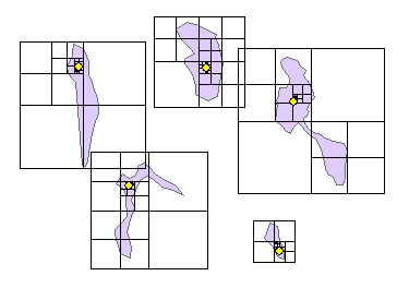
Yesterday, I attempted to replicate the Mapbox Visual Center algorithm using ArcGIS arcpy (Python). Today, I actually looked at the source code (code, license) and attempted to fully port it over from JavaScript. I think it works properly, but you tell me.

def polylabel(polygon, centroid, precision, debug):
    cells = []
    precision = precision or 1.0
    extent = polygon.extent
    minX, minY, maxX, maxY = (extent.XMin, extent.YMin, extent.XMax, extent.YMax)
    width = extent.width
    height = extent.height
    cellSize = min([width, height])
    h = cellSize / 2
    cellQueue = []
    x = minX
    while x < maxX:
        y = minY
        while y < maxY:             cell = Cell(x+h, y+h, h, polygon)             cells.append(cell.geom)             cellQueue.append(cell)             y += cellSize         x += cellSize     bestCell = Cell(centroid[0], centroid[1], 0, polygon)     numProbes = len(cellQueue)     while len(cellQueue):         cellQueue.sort(key=lambda cell: cell.d)         cell = cellQueue.pop()         cells.append(cell.geom)         if cell.d > bestCell.d:
            bestCell = cell
        if cell.max - bestCell.d <= precision:
            continue
        h = cell.h/2
        cellQueue.append(Cell(cell.x-h, cell.y-h, h, polygon))
        cellQueue.append(Cell(cell.x+h, cell.y-h, h, polygon))
        cellQueue.append(Cell(cell.x-h, cell.y+h, h, polygon))
        cellQueue.append(Cell(cell.x+h, cell.y+h, h, polygon))
        numProbes += 4
    return [bestCell.x, bestCell.y, cells]
class Cell():
    def __init__(self, x, y, h, polygon):
        self.x = x
        self.y = y
        self.h = h
        self.d = pointToPolygonDist(x, y, polygon)
        self.max = self.d + self.h * math.sqrt(2)
        self.geom = arcpy.Polygon(arcpy.Array([arcpy.Point(x-h,y-h),arcpy.Point(x+h,y-h),arcpy.Point(x+h,y+h),arcpy.Point(x-h,y+h)]))
def pointToPolygonDist(x, y, polygon):
    point_geom = arcpy.PointGeometry(arcpy.Point(x, y),sr)
    polygon_outline = polygon.boundary()
    min_dist = polygon_outline.queryPointAndDistance(point_geom)
    sign_dist = min_dist[2] * ((min_dist[3]-0.5)*2)
    return sign_dist
fc = 'BEC_POLY selection'
sr = arcpy.Describe(fc).spatialReference
centroids = []
label_points = []
cells = []
with arcpy.da.SearchCursor(fc,['SHAPE@','SHAPE@XY']) as cursor:
    for row in cursor:
        best_point = polylabel(row[0],row[1],.75,'#')
        centroids.append(arcpy.PointGeometry(row[0].centroid,sr))
        label_points.append(arcpy.PointGeometry(arcpy.Point(best_point[0], best_point[1]),sr))
        for cell in best_point[2]:
            cells.append(cell)
arcpy.CopyFeatures_management(centroids,r'in_memory\centroids')
arcpy.CopyFeatures_management(label_points, r'in_memory\label_points')
arcpy.CopyFeatures_management(cells, r'in_memory\cells')

Mapbox Visual Center Algorithm: arcpy

quadtree

On Monday, Mapbox published a JavaScript implementation of a fast algorithm for finding the visual center of a polygon using quadtrees (blog, code). I took a stab at it using Python/arcpy in ArcGIS:

def quadify(poly): # split polygon into quads
    ext = poly.extent
    TM = arcpy.Point((ext.XMin+ext.XMax)/2,ext.YMax)
    LM = arcpy.Point(ext.XMin,(ext.YMin+ext.YMax)/2)
    BM = arcpy.Point((ext.XMin+ext.XMax)/2,ext.YMin)
    RM = arcpy.Point(ext.XMax,(ext.YMin+ext.YMax)/2)
    TL = arcpy.Polygon(arcpy.Array([ext.upperLeft,LM,poly.centroid,TM]),sr)
    TR = arcpy.Polygon(arcpy.Array([TM,poly.centroid,RM,ext.upperRight]),sr)
    BL = arcpy.Polygon(arcpy.Array([LM,ext.lowerLeft,BM,poly.centroid]),sr)
    BR = arcpy.Polygon(arcpy.Array([poly.centroid,BM,ext.lowerRight,RM]),sr)
    return [TL,TR,BL,BR]
def inspect(quad,poly): # calculate quad radius & quad center to polygon distance
    poly_boundary = poly.boundary()
    quad_center = arcpy.PointGeometry(quad.centroid,sr)
    radius = quad_center.distanceTo(quad.firstPoint)
    q_dist = poly_boundary.queryPointAndDistance(quad_center)
    dist = q_dist[2] if q_dist[3] else -q_dist[2]
    return dist + radius
def loop_quads(quads): # evaluate the quads & return if in the top 10% of values
    max_quads = []
    max_dist = 0
    dists = {}
    for quad in quads:
        cur_dist = inspect(quad,row[0])
        dists[cur_dist] = quad
        max_dist = cur_dist if cur_dist > max_dist else max_dist
        out_polys.append(quad)
    for k,v in dists.iteritems():
        if k > max_dist * 0.90: # precision = 90%
            max_quads.append(v)
    return max_quads
fc = 'wetlands_select' # feature class/layer
sr = arcpy.Describe(fc).spatialReference # spatial reference
out_polys = []
out_points = []
with arcpy.da.SearchCursor(fc,'SHAPE@',spatial_reference=sr) as cursor: # loop polygons
    for row in cursor:
        ext = row[0].extent
        center = arcpy.PointGeometry(arcpy.Point((ext.XMin+ext.XMax)/2,(ext.YMin+ext.YMax)/2),sr)
        radius = max(center.distanceTo(ext.upperLeft),center.distanceTo(ext.upperRight),center.distanceTo(ext.lowerLeft),center.distanceTo(ext.lowerRight))
        circle = center.buffer(radius)
        quads = quadify(circle) # start with global circle
        for i in range(10): # quadify 10x
            max_quads = loop_quads(quads) # evaluate current set of quads
            quads = []
            for quad in max_quads:
                quads += quadify(quad)
        out_points.append(arcpy.PointGeometry(quad.centroid,sr)) # return one of the best quad centers
arcpy.CopyFeatures_management(out_polys,r'in_memory\polys')
arcpy.CopyFeatures_management(out_points,r'in_memory\points')

Notes:

I’m not 100% sure that this emulates the base Mapbox algorithm, and I didn’t attempt to implement the “priority queue” enhancement.

The results are somewhat sensitive to the precision factor, but I suppose that’s the be expected with a speed algorithm.

I realize that you can calculate a label point much easier within ArcGIS using out-of-the-box tools. This was just me exploring the algorithm.

Anyhow, I welcome your comments on the code above!

Simple CesiumJS Skydive Sim

skydive

Note: updated version with guidance lights here.

On July 30, 2016, a man named Luke Aikins went skydiving, without a parachute, and landed safely in a net. I was curious what that would feel like, so I made this simple skydiving simulation using CesiumJS.

You can track using W, A, S, D to feel how much control you could possibly have on the descent.

The simulation parameters are as follows:

  • the location is similar to the event, but I’m not exactly sure where it took place. Apparently, it was at the Big Sky movie ranch, near Simi Valley, CA. This is the nearest open area to where Google Maps tells me that is.
  • the red target on the ground is 30m x 30m, same as at the event
  • the simulation starts at 7620m (or 25,000 feet), same as at the event
  • you fall at 53.6448 meters/second, which is 120mph, which is at the slower end of the velocity range a human would travel during free fall. I figure he was trying to go as slow as possible, but there’s only so much you can do to make that happen!
  • I was surprised to learn (simultaneously from both @tkw954 and @erikfriesen – thanks!) that a good skydiver can track at 45 degrees (1:1 glide ratio), which made the math for horizontal movement super-simple – it equals the fall rate.

I stole borrowed most of the animation/control code from the Cesium Camera Tutorial.

The simulation ends in blackness, which is because I was too lazy to make a net, however with no net, that seems fitting. Have fun!

edit (08/06/16): this post was featured on Maps Mania!

edit (08/09/16): added guidance lights to this example. This is likely not how the actual light guidance system worked. In my example, the farther you’re aimed from each corner (up to 100m), the more red the circle turns. The closer you’re aimed to each corner, the more green it turns. It would be more useful to code the lights to indicate in which direction to correct, but I only have so much time.

edit (09/01/16): this post was mentioned in the Cesium Blog!

edit (12/29/16): this post was mentioned in the Exploratorium Blog!

Basic Mapzen/Tangram test

pg_mapzen

Over the past few days, I’ve jumped into the Mapzen/Tangram ecosystem. First impressions: somewhat steep learning curve to grasp YAML format, lighting options are pretty neat, very fast to render GeoJSON, documentation is good although asks a lot of the newbie reader, the provided Mapzen Vector Tile Service (mostly OSM) is awesome, and I bet shaders are cool, but I don’t understand them (yet).

My example is largely based off the Mapzen JS Walkthrough, with a few simple additional wrinkles. I draw parcel geometry and attribute data directly from Open Data Prince George. I take building data from the same source, remove OSM buildings from the scene, and draw/extrude 3D buildings based on the building height attribute.

Antipodes (MapboxGL)

antipodes

In 2013, I made an interactive antipode map (points on opposite sides of the Earth) using the Google Maps API. As I’m trying to make the leap from Google Maps/Mapbox JS to Mapbox GL JShere is my rehash of the same map. The only tangible difference between these two maps is that you can rotate this version (right-click and drag).

Some issues I have yet to solve:

  • I can’t seem to get the rotated maps’ labels to display correctly (i.e. right-side up and left to right). I would need to somehow change them to be rendered as a mirror image.
  • The second set of maps don’t render at all in Chrome, although they do while testing locally. This entire project seems to work in IE and Firefox. edit: this project now seems to work in Chrome.

– this map was featured on Google Maps Mania! http://googlemapsmania.blogspot.ca/2016/07/the-antipodes-maps.html


Draggable Latitude Line Map

latline

I just returned home from a trip to Scandinavia (Denmark/Sweden/Norway), and was curious to see how far north I’d gone. I made it as far as Tromsø, which is at about 69.7°N, but where would that latitude place me in North America? It turns out, pretty far north – about halfway up Baffin Island. See for yourself on this quick map (drag the marker to move the line north and south, then see where in the world passes through that latitude).

Old Prince George Floodplain Map

flood

Just thought I’d share a cool looking old map overlay I found digging through the BC Map Services. I enjoy the very detailed, yet simple look. I’ve also superimposed the City of Prince George Flood Plain 1997 layer, which I think is the digitized version of the scanned BC map. Kinda scary to see how far up Patricia/Winnipeg/17th/Massey it would flood, but I guess the City’s got it figured out.